Input Database Constituent File Details

General Database File Structure

The .csv files featured below collectively represent the EP input database. Each file and its contents are explained in detail in Section 5.3. Section headers are included before file names for reference.

• Geographies

  • GeographiesSpatialJoin.csv

  • Geographies.csv

  • GeographiesMapKeys.csv

• Drivers

  • DemandDrivers.csv

• Subsector Data Input: Energy Demand Method

  • Demand Itself: DemandEnergyDemands.csv

  • Energy Efficiency Measures (e.g., 1% annual efficiency growth)

    • DemandEnergyEfficiencyMeasures.csv

    • DemandEnergyEfficiencyMeasuresCost.csv

  • Fuel Switching Measures (e.g., force a switch from gasoline to electricity)

    • DemandFuelSwitchingMeasures.csv

    • DemandFuelSwitchingMeasuresCost.csv

    • DemandFuelSwitchingMeasuresEnergyIntensity.csv

    • DemandFuelSwitchingMeasuresImpact.csv

• Subsector Data Input: Stock and Service Method

  • Service Demand

    • DemandSerivceDemands.csv

    • DemandServiceDemandMeasures.csv

    • DemandServiceDemandMeasuresCost.csv

    • DemandServiceEfficiency.csv

    • DemandServiceLink.csv

  • Technology Stock/Sales

    • DemandStock.csv

    • DemandStockMeasures.csv

    • DemandSales.csv

    • DemandSalesShareMeasures.csv

  • Technology Details

    • DemandTechs.csv

    • DemandTechsAirPollution.csv

    • DemandTechsAuxEfficiency.csv

    • DemandTechsCapitalCost.csv

    • DemandTechsFixedMaintenanceCost.csv

    • DemandTechsFuelSwitchCost.csv

    • DemandTechsIncentive.csv

    • DemandTechsInstallationCost.csv

    • DemandTechsMainEfficiency.csv

    • DemandTechsParasiticEnergy.csv

    • DemandTechsSerivceDemandModifier.csv

    • DemandTechsServiceLink.csv

• Energy Demand Temporal Patterns

  • Shapes.csv

  • ShapeData folder (energy demand temporal patterns)

    • E.g., residential_electricity.csv contains residential electricity demand for every hour of the year for different geographical regions.

  • DispatchFeedersAllocation.csv

• Other

  • DemandSectors.csv

  • DemandSubsectors.csv

  • FinalEnergy.csv

  • CurrenciesConversion.csv

  • InflationConversion.csv

  • OtherIndexes.csv

Common Terms in Database Files

The following terms appear in multiple database files and are defined here to avoid redundancy. Other terms that are uniquely used in only one database file are defined in the section of this reposit where that file is explicated.

• age_growth_or_decay_type: This control allows quantities to grow or decay over the lifetime of a technology. For example, a vintage 2030 gasoline car (a car that entered the technology stock in 2030) may experience a loss in efficiency as it ages. The initial efficiency value in 2030 < the value in 2031 < the value in 2032… The two options for this decay type are “linear” and “exponential.” Respective growth rates are specified in age­_growth_or_decay, described in the next term.

  • It is important to understand that this control influences how a vintage of technology changes across its lifetime. For instance, in the efficiency example above, this control does not influence the efficiency of new gasoline cars sold over time. It only controls how the efficiency of a car added to the stock in year “x” changes as that vintage car enters year “x+1”, “x+2,” … of its lifespan.

• age_growth_or_decay: This control specifies the rate at which quantities change over the lifetime of the technology according to the “linear” or “exponential” function specified in age_growth_or_decay_type.

  • If the “exponential” type is selected, this value is the yearly rate of change. For example, “0.01” indicates a growth of 1% each year. Similarly, “-0.01” indicates a decay of 1% each year.

  • If the “linear” type is selected, this value is what portion of the initial value the function increases or decreases by each year. For example, a value of “0.01” indicates that the quantity increases linearly by 1% of the initial value each year. If the initial efficiency value is 10 miles per gallon and a value of “0.01” is selected, the efficiency value would linearly increase by 0.01 x 10 = 0.1 miles per gallon each year.

• cost_denominator_unit: cost is in $/x. What is x? (e.g., GJ for gigajoules)

• cost_of_capital: Weighted Average Cost of Capital (WACC) (in decimal value)

• demand_technology: a technology that uses energy to provide a service (e.g., an electric vehicle, a gasoline vehicle, a refrigerator, a heat pump, etc.)

• driver_1

• driver_2

• driver_3

  • Relevant drivers (if any) for projections, as explained in Section 4.2.

• driver_denominator_1

• driver_denominator_2

  • indicates the driver that a data input has been normalized by. For example, light duty vehicle service demand may be input as annual vehicle miles traveled per person. In this case, the driver denominator would be ‘population’.

• extrapolation_method: method used to extrapolate data beyond range of years explicitly defined in the database. (same input options as interpolation_method, featured below)

• extrapolation_growth: if (and only if) the “exponential_interpolation” method is specified in extrapolation_method, the user can specify a growth rate for extrapolated values here. For example, putting 0.01 for extrapolation_growth will force a 1% increase in extrapolated values each year. Otherwise, the interpolated curve from the previous two data points will be projected forward to obtain extrapolated values.

• final_energy: final-energy type of data input (any from list in FinalEnergy.csv – see Section FinalEnergy.csv)

• gau: ‘geographical analysis unit’ – references a single zone within a geography category.

  • E.g., Within a geography of “state,” each individual state (e.g., “new jersey”) is a gau.

  • There is a special hardcoded geography-gau pair of “global” (geography) and “all” (gau) used for data inputs that cover all geographical regions (e.g., national level data for Australia).

• geography: geographical category of data input (e.g., state, province, city)

• geography_map_key: used to upscale or downscale data inputs between geographies.

  • E.g., if iron and steel sector energy demand is taken in on the national level, but the model is run on the state level, the demand may be broken down by state in proportion to the map key of steel production. See additional discussion in Section Geographies.

• input_type: specifies that input data is an “intensity” or “total” value. (these are the only two options)

  • E.g., is the data for all people (total) or per person (intensity)?

• interpolation_method: method used to interpolate data between given years (e.g., if data is given for 2030 and 2040, how do we get data for 2035?) See list of options below. Figure below offers a visual description for several of the methods.

  • linear_interpolation: Adjacent data points are connected with a line to generate missing data.

  • linear_regression: A line of best fit is generated from all provided data points. Original data are replaced with data along this line. Missing data are found from this line. (i.e., all data is along a line of best fit)

  • logistic: Fits an s-curve function to the provided data points. Original data are replaced with data along this curve, and missing data are found from the curve.

  • cubic: Fits a cubic spline to the provided data points using the scipy library. The spline contains all the provided data points, and missing data are found along the spline.

  • quadratic: Fits a quadratic spline to the provided data points using the scipy library. The spline contains all provided data points, and missing data are found along the spline.

  • nearest: Missing data are filled to be equal to the nearest provided data point.

  • exponential_interpolation: Adjacent data points are connected with an exponential curve to generate missing data, similar to how linear interpolation works but exponential curves instead of straight lines. In extrapolation, there is no final point to connect a curve to. The model will use the previous curve (from the previous two points) and project it forward unless an exponential growth rate is given in the extrapolation_growth column. A value of 0.01 given in the extrapolation_growth column forces 1% annual growth in extrapolated values.

  • exponential_regression: Creates a best fit exponential curve for all the provided data points using the polyfit function. Original data are replaced with data along this curve. Missing data are found from the curve.

  • average: replaces provided values with a mean (flat line at mean value).

  • decay_towards_linear_regression: Only an option for extrapolation. After the final provided data point, values approach the line of best fit (the same line used in linear_regression method).

  • forward_fill: missing years are made equal to the closest historical year.

  • back_fill: missing years are made equal to the closest future year.

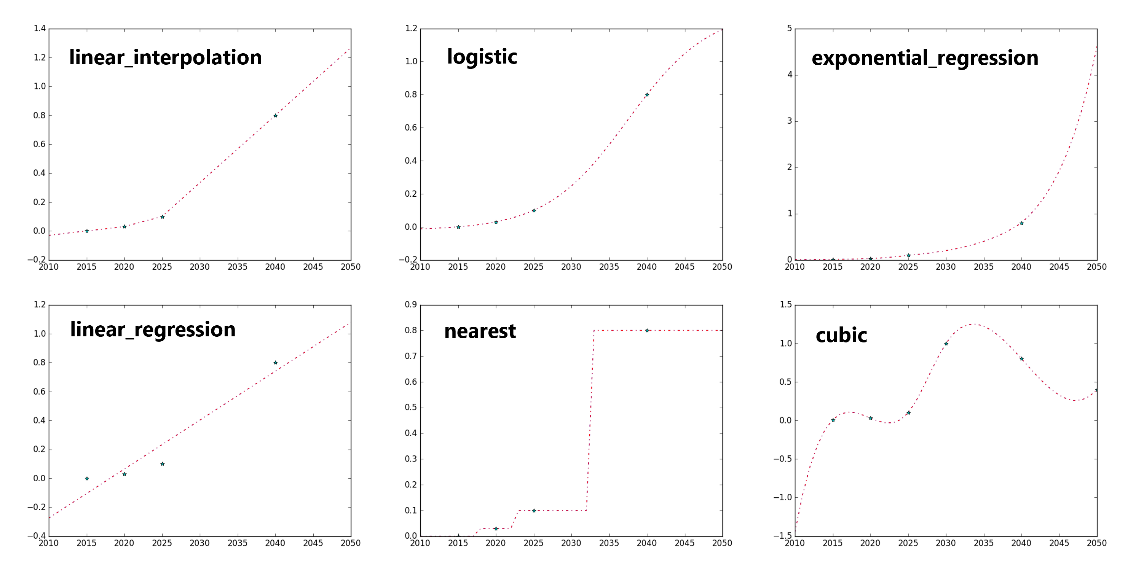
Graphical example of several interpolation/extrapolation methods. Provided data points are blue stars. Source: EnergyPATHWAYS Model Website.

• is_levelized: is the capital cost annualized? (TRUE/FALSE)

• is_stock_dependent: is total service demand dependent on size of stock? (TRUE or FALSE)

• lifetime_variance: variance in lifetime of a technology in years

  • Note: user must either specify min and max lifetime or mean and variance

• max_lifetime: maximum lifetime of technology in years

  • Note: user must either specify min and max lifetime or mean and variance

• mean_lifetime: mean lifetime of technology in years

  • Note: user must either specify min and max lifetime or mean and variance

• min­_lifetime: minimum lifetime of technology in years

  • Note: user must either specify min and max lifetime or mean and variance

• notes: user notes to document assumptions (not used for computations in model)

• other_index_1

• other_index_2

  • Optional additional index categories to maintain during calculations, e.g., in the residential sector, building type can be an additional level of grouping data and viewing results.

  • See the description of OtherIndexes.csv (Section OtherIndexes.csv) for more information on other indexes.

• oth_1: one element from the other_index_1 category. Ex. If other_index_1 is ‘building_type’, oth_1 may be ‘detached single family’.

• oth_2: analogous to oth_1 for other_index_2

• sector: main groupings of energy consumption (e.g., in Net Zero Australia, these are productive, commercial, residential, and transportation)

• sensitivity: sensitivity tag for the data input

  • E.g., for 2040 population, may have a high, medium, and low estimate depending on sensitivity (“low”, “medium [d]”, “high”)

  • [d] indicates default option for model to select (if not specified in runs_key file)

• shape: hourly shape of the service demand for a sector, subsector, or technology

  • e.g., commercial_electricity, industry_electricity (productive sector), residential_elecricity

• source: where the data/information came from (not used in model calculations)

• stock_decay_function: models the rate at which vintaged stock decays and needs to be replaced. Three options are “linear,” “exponential,” and “weibull.” See Section Stock Rollover Calculation for more information on the stock rollover calculations.

• subsector: sub-groupings of energy consumption (e.g., in Net Zero Australia, subsectors of the productive sector are specific industries, like the iron and steel industry).

• vintage: sales year of technology

Database File-by-File Details

This section explores every database file, its purpose, and contents. Column headers without a description are featured as common terms in Section Common Terms in Database Files.

GeographiesSpatialJoin.csv

Purpose: Fundamental geography table. Indicates relevant geography types (geography), names (gau), time zones, and map keys to scale data between different granularities.

Figure below depicts a sample spatial join table for a preliminary China study. The column headers circled in red are the geography types (geography). In this case, data is only input on the national or provincial level. The analysis units (gau) associated with each type are listed below the headers. These include each individual province as well as the country as a whole (“china”). The column headers circled in blue are map keys (e.g., population, land area, occupied dwellings, steel production) with values for each region listed below them. Time zones are chosen from the time_zones.csv file that was installed from GitHub with the EnergyPATHWAYS model. It is featured in the energyPATHWAYS folder of the installation.

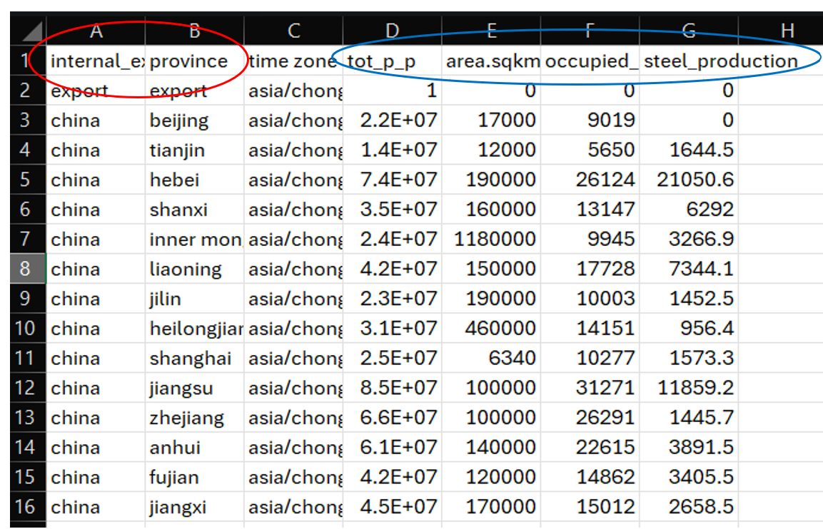
Sample geography spatial join table for a China study. Geography types are circled in red. Geography map keys are circled in blue.

Geographies.csv

Purpose: List relevant geographic types (geography) and regions (gau) for use in the database and model run.

Column Breakdown:

1. geography

2. gau

GeographyMapKeys.csv

Purpose: List relevant geography map keys for scaling data cross granularities.

Column Breakdown:

1. name: map key name (e.g., steel production 2023)

DemandDrivers.csv

Purpose: factors used to project energy and service demands over time. E.g., population, gross domestic product, square footage of commercial building types, vehicle miles traveled.

Column Breakdown:

1. name: driver name

2. base driver: is the driver specified in column A tied to a more fundamental driver?

   1. E.g., a driver of households may have a base driver of population. To project household size into the future, the method explained in Section Demand Drivers will be used, with the driver being population.

3. input_type

4. unit_prefix: value of a single unit

   1. E.g., does a value of “1” represent 1 person, 2 people, 3 people?

5. unit_base: what is the unit in question?

   1. E.g., people, households, square meters of floor

6. geography

7. other_index_1

8. other_index_2

9. geography_map_key

10. interpolation_method

11. extrapolation_method

12. extrapolation_growth

13. source

14. notes

15. gau

16. oth_1

17. oth_2

18. year: year of data input

19. value: demand driver value (in relative or absolute units, as specified in Columns C-E)

    1. E.g., annual population value

20. sensitivity

DemandEnergyDemands.csv

Purpose: Accounts for energy demand in subsectors without enough information for a stock/service demand calculation.

Column Breakdown:

1. subsector

2. is_stock_dependent

3. input_type

4. unit

5. driver_denominator_1

6. driver_denominator_2

7. driver_1

8. driver_2

9. driver_3

10. geography

11. final_energy_index: generally blank but unsure of exact purpose

12. demand_technology_index: generally blank but unsure of exact purpose

13. other_index_1

14. other_index_2

15. interpolation_method

16. extrapolation_method

17. extrapolation_growth

18. geography_map_key

19. source

20. notes

21. gau

22. oth_1

23. oth_2

24. final_energy

25. demand_technology

26. year

1. value: energy demand value for subsector (Column A), year (Column Z), and energy type (Column X) specified

AB. sensitivity

DemandEnergyEfficiencyMeasures.csv

Purpose: Allows user to change energy efficiency over time for subsectors that run with the simple energy demand method (those in DemandEnergyDemands.csv).

Column Breakdown:

1. name: measure name (a specific name like “DDP: food; beverages and tobacco” is helpful for understanding what is represented; DDP stands for “Deep Decarbonization Pathway” as opposed to REF which stands for “Reference.”)

2. subsector

3. input_type: efficiencies are always an intensity

4. unit: energy efficiencies are generally unitless (blank box)

5. geography

6. other_index_1

7. other_index_2

8. interpolation_method

9. extrapolation_method

10. extrapolation_growth

11. stock_decay_function: not used/outdated

12. min­_lifetime: not used/outdated

13. max_lifetime: not used/outdated

14. mean_lifetime: not used/outdated

15. lifetime_variance: not used/outdated

16. source

17. notes

18. final_energy

19. gau

20. oth_1.

21. oth_2

22. year

23. value: energy efficiency gain by year specified. For example, a typical value is 0.310550914 in 2060 and 0 in 2023. This represents 1% annual efficiency gain from 2023 to 2060, since 1-0.99^2060-2023 = 0.310550914. The interpolation­_method is used to fill in values for the intermediate years.

DemandEnergyEfficiencyMeasuresCost.csv

Purpose: Specification of the cost of induced efficiency improvement measures specified in DemandEnergyEfficiencyMeasures.csv.

Column Breakdown:

1. parent: measure name (from DemandEnergyEfficiencyMeausures.csv)

2. currency

3. currency_year

4. cost_denominator_unit

5. cost_of_capital

6. is_levelized

7. geography

8. other_index_1

9. other_index_2

10. interpolation_method

11. extrapolation_method

12. extrapolation_growth

13. source

14. notes

15. gau

16. oth_1

17. oth_2

18. vintage

19. value: cost of induced efficiency improvement measure in units of currency/cost_denominator_unit (e.g., 10 $/GJ)

20. final_energy: (empty for NZAu)

DemandFuelSwitchingMeasures.csv

Purpose: Allows user to control energy type (ex. force a transition from coal to electricity) in sectors that run with the simple energy demand method (those in DemandEnergyDemands.csv).

Column Breakdown:

1. name: measure name (a specific name like “DDP: food; beverages and tobacco” is helpful for understanding what is represented; DDP stands for “Deep Decarbonization Pathway” as opposed to REF which stands for “Reference.”)

2. subsector

3. final_energy_from: original energy type (e.g., diesel)

4. final_energy_to: new energy type (e.g., electricity)

5. stock_decay_function

6. min­_lifetime

7. max_lifetime

8. mean_lifetime

9. lifetime_variance

DemandFuelSwitchingMeasuresCost.csv

Purpose: Incorporate cost of fuel switching measures specified in DemandFuelSwitchingMeasures.csv.

Column Breakdown:

1. parent: measure name (from DemandFuelSwitchingMeasures.csv)

2. currency

3. currency_year

4. cost_denominator_unit

5. cost_of_capital

6. is_levelized

7. geography

8. other_index_1

9. other_index_2

10. interpolation_method

11. extrapolation_method

12. extrapolation_growth:

13. source

14. notes

15. gau

16. oth_1

17. oth_2

18. vintage

19. value: cost of fuel switching measure in units of currency/cost_denominator_unit (e.g., 10 $/GJ)

DemandFuelSwitchingMeasuresEnergyIntensity.csv

Purpose: Specify change in energy intensity as a result of fuel switching measures specified in DemandFuelSwitchingMeasures.csv.

Column Breakdown:

1. parent: measure name (from DemandFuelSwitchingMeasures.csv)

2. geography

3. other_index_1

4. other_index_2

5. interpolation_method

6. extrapolation_method

7. extrapolation_growth

8. source

9. notes

10. gau

11. oth_1

12. oth_2

13. year

14. value: new energy intensity (relative to original fuel). For example, 0.5 indicates that total energy demand for this process/subsector dropped by 50% as a result of switching fuels. This could represent switching from coal blast furnaces to electric arc furnaces (EAFs) in the iron and steel sector, since EAFs consume less energy to produce the same amount of steel.

DemandFuelSwitchingMeasuresImpact.csv

Purpose: Allow users to control rate at which fuel switching measures in DemandFuelSwitchingMeasures.csv occur.

Column Breakdown:

1. parent: measure name (from DemandFuelSwitchingMeasures.csv)

2. input_type: intensities are always an intensity

3. unit: intensities are generally unitless (blank box)

4. geography

5. other_index_1

6. other_index_2

7. interpolation_method

8. extrapolation_method

9. extrapolation_growth

10. source

11. notes

12. gau

13. oth_1

14. oth_2

15. year

16. value: what proportion of old fuel has been replaced by new fuel in year specified

    1. Ex. 0 indicates no replacement. 0.5 indicates 50% replacement of old fuel use with new fuel. 1 indicates full replacement of old fuel use with new fuel.

DemandServiceDemands.csv

Purpose: Outline annual service demands and projection methods.

Column Breakdown:

1. subsector

2. is_stock_dependent

3. input_type

4. unit: demand unit, e.g., available_seat_kilometer

5. driver_denominator_1

6. driver_denominator_2

7. driver_1

8. driver_2

9. driver_3

10. geography

11. final_energy_index: generally blank but unsure of exact purpose

12. demand_technology_index: generally blank but unsure of exact purpose

13. other_index_1

14. other_index_2

15. interpolation_method

16. extrapolation_method

17. extrapolation_growth

18. geography_map_key

19. source

20. notes

21. gau

22. final_energy

23. demand_technology

24. oth_1

25. oth_2

26. year

1. value: service demand value

AB. sensitivity

DemandServiceDemandMeasures.csv

Purpose: Allow user to alter the projection of service demand in a subsector. For example, if we project a 25% decline in vehicle miles traveled, we could enter that as a measure here.

Column Breakdown:

1. name: measure name (user is recommended to use informative name like “DDP_lowdemand: commercial air conditioning”)

2. subsector

3. input_type

4. unit

5. geography

6. other_index_1

7. other_index_2

8. interpolation_method

9. extrapolation_method

10. extrapolation_growth

11. stock_decay_function: not used/outdated

12. min­_lifetime: not used/outdated

13. max_lifetime: not used/outdated

14. mean_lifetime: not used/outdated

15. lifetime_variance: not used/outdated

16. geography_map_key

    1. Blank for NZAu

17. source

18. notes

19. gau

20. oth_1

21. oth_2

22. year

23. value: relative service demand growth (relative to 2020 baseline (0) in Australia)

    1. e.g., value of 0.2 in 2050 and 0 in 2020 indicates a 20% decline in service demand from 2020-2050.

DemandServiceDemandMeasuresCost.csv

Purpose: Incorporate cost of service demand measures specified in DemandServiceDemandMeasures.csv.

Column Breakdown: *Note: Empty spreadsheet for NZAu

1. parent: relevant service measure

2. currency

3. currency_year

4. cost_denominator_unit

5. cost_of_capital

6. is_levelized

7. geography

8. other_index_1

9. other_index_2

10. interpolation_method

11. extrapolation_method

12. extrapolation_growth

13. source

14. notes

15. gau

16. oth_1

17. oth_2

18. vintage

19. value: cost of service demand measure in units of currency/cost_denominator_unit (e.g., $/km)

DemandServiceEfficiency.csv

Purpose: Allows for input of service efficiency for subsectors that run on the Service Demand and Efficiency method (when not enough information available for full stock rollover calculation).

Column Breakdown:

1. subsector: only used for “cement CO2 capture” for NZAu

2. energy_unit: ex. mmbtu

3. denominator_unit: ex. tonne (mmbtu/tonne overall unit)

4. geography

5. other_index_1

6. other_index_2

7. interpolation_method

8. extrapolation_method

9. extrapolation_growth

10. geography_map_key

11. source

12. notes

13. final_energy

14. gau

15. oth_1

16. oth_2

17. year

18. value: service efficiency in units of energy_unit/denominator_unit (e.g., J/km)

19. sensitivity

DemandServiceLink.csv

Purpose: Specify relationships in service demand between subsectors. For example, the user can control what percentage of hot water service demand comes from clothes washing. Thus, if service demand for clothes washing drops, hot water service demand also drops according to the service demand ratio.

Column Breakdown:

1. name: user-created name of service demand linkage (e.g., “dem_svc_link_1”, “dem_svc_link_2,” …)

2. subsector: affecting subsector (e.g., if clothes washing contributes to hot water demand, clothes washing would be the affecting subsector since it affects hot water demand)

3. linked_subsector: affected subsector (e.g., if clothes washing contributes to hot water demand, hot water would be the affected subsector since its service demand was impacted by clothes washing service demand.)

4. service_demand_share: Value is ratio of shared service demand. For example, If the subsector is “residential clothes washing” and the linked subsector is “residential water heating,” a value of “0.25” specifies that 25% of hot water demand is from clothes washing. So, if clothes washing goes down 100% in service demand (is eliminated), hot water service demand drops 25%.

5. year

DemandStock.csv

Purpose: Define stock of technologies for each subsector.

Column Breakdown:

1. subsector

2. is_stock_dependent

3. driver_denominator_1

4. driver_denominator_2

5. driver_1

6. driver_2

7. driver_3

8. geography: geographical category of data input

9. other_index_1

10. other_index_2

11. geography_map_key

12. input_type

13. demand_stock_unit_type: unit type (generally “equipment”)

14. unit: stock unit (ex. truck)

15. time_unit: if time is relevant to stock unit

16. interpolation_method

17. extrapolation_method

18. extrapolation_growth

19. specify_stocks_past_current_year: do you want to specify stock past the current year? (ex. specify 2050 stock breakdown) (TRUE/FALSE)

20. source

21. notes

22. gau

23. oth_1

24. oth_2

25. demand_technology

26. year

1. value: stock quantity

AB. sensitivity

DemandStockMeasures.csv

Purpose: Allows user to directly control stock composition (as opposed to sales measures) (only used for “2017 AEO Res Distillate Boiler” in NZAu)

Column Breakdown:

1. name: technology name

2. subsector

3. geography

4. other_index1

5. demand_technology

6. interpolation_method

7. extrapolation_method

8. extrapolation_growth

9. source

10. notes

11. gau

12. oth_1

13. year

14. value: stock size in year specified (only zeros used in NZAu)

DemandSales.csv

Purpose: If there are no technological classifications of historical stock data, the model will not know how to replace decayed technology in the baseline rollover (the rollover without the use of any sales share measures). An input to DemandSales.csv specifies this baseline rollover rate.

Column Breakdown:

1. subsector

2. geography

3. other_index_1

4. other_index_2

5. input_type

6. interpolation_method

7. extrapolation_method

8. extrapolation_growth

9. source

10. notes

11. gau

12. oth_1

13. oth_2

14. demand_technology

15. vintage

16. value: proportion of sales made up by demand­_technology (Column N) in vintage year (Column O).

17. sensitivity

DemandSalesShareMeasures.csv

Purpose: Directly control sales rates in a certain year (e.g., can specify what percent of cars sold in 2050 are EVs) to influence stock.

Column Breakdown:

1. name: measure name (a descriptive name is helpful. For example, “REF: CFL Exterior -> Incandescent Exterior” is referring to the replacement rate of decayed incandescent exterior lights with new CFL exterior lights in the reference case.)

2. subsector

3. geography

4. other_index_1

5. demand_technology: new technology

   1. e.g., CFL Exterior for example in A

6. replaced_demand_tech: technology that decayed and will be replaced by demand_technology

   1. e.g., Incandescent Exterior for example in A

7. input_type

8. interpolation_method

9. extrapolation_method

10. extrapolation_growth

11. source

12. notes

13. gau

14. oth_1

15. vintage

16. value: what proportion of sales in subsector are for demand_technology? If replacing, what proportion of replaced_demand_tech should be replaced by demand_technology upon decay in stock rollover?

DemandTechs.csv

Purpose: Specify relevant demand technologies for the model. A demand technology is a device that uses energy to meet a service demand.

Column Breakdown:

1. name: relevant technology (e.g., Electric Transit Bus)

2. linked: technology that the current technology is linked to. For example, a heat pump that provides heating is also linked to a heat pump that provides cooling.

3. stock_link_ratio: controls ratio of stock between linked technologies

4. subsector

5. source

6. additional_description: user notes (not used by model)

7. demand_tech_unit_type: technology unit type (only “equipment” used in NZAu)

8. unit: technology unit (e.g., bus, truck, motorcycle)

9. time_unit: time unit if relevant (blank for NZAu)

10. cost_of_capital

11. stock_decay_function

12. min_lifetime

13. max_lifetime

14. mean_lifetime

15. lifetime_variance

16. shape

DemandTechsAirPollution.csv

Purpose: Specify air pollutant emissions for technologies listed in DemandTechs.csv.

Column Breakdown:

1. demand_technology

2. definition: is the value “absolute” or “relative” to another demand technology

3. reference_tech: reference technology (if definition is relative)

4. mass_unit: unit of mass for pollutant ex. kilogram

5. energy_unit: ex. mmbtu

6. geography

7. other_index1: “air pollution” for this data sheet

8. other_index2: blank for this sheet

9. interpolation_method

10. extrapolation_method

11. extrapolation_growth

12. source

13. notes

14. gau

15. oth_1: specific pollutant for this data row (ex. Nox, PM2.5, Sox)

16. oth_2: blank for this sheet

17. final_energy

18. vintage

19. year

20. value: pollutant value in units of mass_unit/energy_unit (ex. 0.35 kg Nox/mmbtu for gasoline LDV vintage 1960 in 1990 Australia)

21. sensitivity

DemandTechsCapitalCost.csv

Purpose: Specification of capital costs for demand technologies listed in DemandTechs.csv.

Column Breakdown:

1. demand_technology

2. definition: absolute or relative

   1. If “relative” definition, specify a reference technology in column C and a conversion operation in column M. For example, an operation of “multiply” in column M will multiply the reference technology’s value by the relative value in column U to obtain this technology’s absolute value.

3. reference_tech

4. geography

5. other_index_1

6. other_index_2

7. currency

8. currency_year

9. is_levelized

10. interpolation_method

11. extrapolation_method

12. extrapolation_growth

13. reference_tech_operation: only “multiply” used in NZAu.

14. source

15. notes

16. new_or_replacement: is technology cost in column U for a “new” installation or “replacement” for a decayed technology? (replacements may have lower costs)

17. gau

18. oth_1

19. oth_2

20. vintage

21. value: see note under B for specifics on relative value (relative to specified reference technology by operation specified in M)

22. sensitivity

DemandTechFixedMaintenanceCost.csv

Purpose: Specification of maintenance costs for demand technologies listed in DemandTechs.csv.

Column Breakdown:

1. demand_technology

2. definition: “absolute” or “relative” (relative to reference technology in column C)

3. reference_tech

4. geography

5. other_index_1

6. other_index_2

7. currency

8. currency_year

9. interpolation_method

10. extrapolation_method

11. extrapolation_growth

12. age_growth_or_decay_type

13. age_growth_or_decay

14. additional_description: same as notes

15. source

16. notes

17. gau

18. oth_1

19. oth_2

20. vintage

21. value: cost value in absolute units or relative to reference technology, as specified by Column B

22. sensitivity

DemandTechsFuelSwitchCost.csv

Purpose: Specification of fuel switching costs for demand technologies listed in DemandTechs.csv.

Column Breakdown:

1. demand_technology

2. definition: absolute or relative (to reference technology specified in column C)

3. reference_tech

4. geography

5. other_index_1

6. other_index_2

7. currency

8. currency_year

9. is_levelized

10. interpolation_method

11. extrapolation_method

12. extrapolation_growth

13. source

14. notes

15. gau

16. oth_1

17. oth_2

18. vintage

19. value: fuel switch cost in absolute units or relative to reference tech, as specified in Column B

20. sensitivity

DemandTechsIncentive.csv

Purpose: Specification of incentives for demand technologies listed in DemandTechs.csv (blank for NZAu study)

Column Breakdown:

1. demand_technology

2. incentive_type: no examples to base on in NZAu

3. apply_lesser_of_incentives

4. include_capital_cost: TRUE/FALSE

5. include_installation_cost: TRUE/FALSE

6. include_fuel_switching_cost: TRUE/FALSE

7. source

8. notes

9. geography

10. other_index_1

11. other_index_2

12. currency

13. currency_year

14. is_levelied

15. interpolation_method

16. extrapolation_method

17. extrapolation_growth

18. gau

19. oth_1

20. oth_2

21. vintage

22. value (in units of currency?)

23. sensitivity

DemandTechsInstallationCost.csv

Purpose: Specify installation costs for demand technologies listed in DemandTechs.csv.

Column Breakdown:

1. demand_technology

2. definition: absolute or relative (to reference technology in C)

3. reference_tech

4. geography

5. other_index_1

6. other_index_2

7. currency

8. currency_year

9. is_levelized

10. interpolation_method

11. extrapolation_method

12. extrapolation_growth

13. source

14. notes

15. new_or_replacement: is technology new or replacing an existing technology?

16. gau

17. oth_1

18. oth_2

19. vintage

20. value: installation cost in currency specified (and absolute or relative units as specified in Column B)

21. sensitivity

DemandTechsMainEfficiency.csv

Purpose: Specify primary efficiencies of demand technologies listed in DemandTechs.csv.

Column Breakdown:

1. demand_technology

2. definition: absolute or relative (to reference technology in C)

3. reference_tech

4. geography

5. other_index_1

6. other_index_2

7. final_energy

8. utility_factor: energy carrier utility factor. This value allocates a share of a technology’s service demand to a specific energy type. For example, a dual fuel technology might use one fuel with one efficiency value half the time and another fuel with a different efficiency value the rest of the time. In this case, the technology would have one line in DemandTechsMainEfficiency.csv and another line in DemandTechsAuxEfficiency.csv to account for both efficiency values. The utility factor x service demand will determine how much of the service demand is met by the “main” efficiency and energy type. The remaining service demand is allocated to the “auxiliary” efficiency and energy type. See Net Zero America Annex A.2, 2020, p. 54 for more information.

9. is_numerator_service: TRUE/FALSE - is numerator (instead of denominator) the service unit?

   1. Ex: lightbulb service demand is in lumens. Efficiency is recorded in lumens/watt. Therefore, the numerator (lumens) is the service unit à TRUE.

   2. Counter-Ex: refrigerator service demand is cubic feet. Efficiency is recorded in kwh/cubic foot. Therefore, the denominator (cubic feet) is the service unit à FALSE

10. numerator_unit: ex. if efficiency in lumens/watt, numerator_unit is lumen or lumen_hour

11. denominator_unit ex. if efficiency in lumens/watt, deominator_unit is watt or watt_hour

12. interpolation_method

13. extrapolation_method

14. extrapolation_growth

15. age_growth_or_decay_type

16. age_growth_or_decay

17. geography_map_key

18. source

19. notes

20. gau

21. oth_1

22. oth_2

23. vintage

24. value: efficiency value in units of numerator_unit/denominator_unit

25. sensitivity

DemandTechsAuxEfficiency.csv

Purpose: Secondary efficiency specification for technologies with two relevant efficiencies (e.g., dual fuel technologies). See note under utility_factor in Section DemandTechsMainEfficiency.csv for more information.

Column Breakdown:

1. demand_technology

2. definition: absolute for both technologies used in NZAu

3. reference_tech: reference technology specification for a non-reference technology (blank for NZAu study)

4. geography

5. other_index_1

6. other_index_2

7. final_energy

8. demand_tech_efficiency_types: blank in NZAu

9. is_numerator_service: TRUE/FALSE - is numerator (instead of denominator) the service unit?

   1. E.g., lightbulb service demand is in lumens. Efficiency is recorded in lumens/watt. Therefore, the numerator (lumens) is the service unit à TRUE.

   2. Counter-Example: refrigerator service demand is cubic feet. Efficiency is recorded in kwh/cubic foot. Therefore, the denominator (cubic feet) is the service unit à FALSE

10. numerator_unit: ex. if efficiency in lumens/watt, numerator_unit is lumen

11. denominator_unit ex. if efficiency in lumens/watt, deominator_unit is watt

12. interpolation_method

13. extrapolation_method

14. extrapolation_growth

15. age_growth_or_decay_type

16. age_growth_or_decay

17. shape

18. source

19. notes

20. gau

21. oth_1

22. oth_2

23. vintage

24. value: auxiliary efficiency value in units of numerator_unit/denominator_unit

    1. if numerator_unit = denominator_unit (e.g., both btu), then efficiency is unitless

25. sensitivity

DemandTechsParasiticEnergy.csv

Purpose: Factor in parasitic energy losses for technologies listed in DemandTechs.csv. Parasitic energy loss is energy that the technology produces that does not directly contribute to meeting service demand. In NZAu, this sheet was only used for Heat Pump and Natural Gas Furnace. Why can we not just factor this into efficiency?

Column Breakdown:

1. demand_technology

2. definition: absolute or relative (to reference technology in C)

3. reference_tech

4. geography

5. other_index_1

6. other_index_2

7. energy_unit

8. time_unit

9. interpolation_method

10. extrapolation_method

11. extrapolation_growth

12. age_growth_or_decay_type

13. age_growth_or_decay

14. source

15. notes

16. gau

17. oth_1

18. oth_2

19. final_energy

20. vintage

21. value: energy loss rate in units of energy_unit/time_unit

22. sensitivity

DemandTechsServiceDemandModifier.csv

Purpose: Without service demand modifiers, service demand is allocated to technologies in proportion to stock. This input allows the user to control how technologies in DemandTechs.csv absorb the service demand (e.g., new cars are driven more than old cars).

Column Breakdown:

1. demand_technology

2. geography

3. definition: absolute or relative (to reference technology in D)

4. reference_tech

5. other_index_1

6. other_index_2

7. interpolation_method

8. extrapolation_method

9. extrapolation_growth

10. source

11. notes

12. gau

13. oth_1

14. oth_2

15. vintage

16. year

17. value: Without service demand modifiers, service demand is allocated to technologies in proportion to stock. This value is a weighting factor for allocating service demand to technology stock. See Net Zero America Annex A.2, 2020, p. 49 for use in equation and p. 52-54 for more information on service demand modifiers.

18. Sensitivity

DemandTechsServiceLink.csv

Purpose: Ryan Jones will follow-up on this control.

Column Breakdown:

1. Name

2. service_link

3. demand_technology

4. definition: all absolute in NZAu study

5. reference

6. geography

7. other_index_1

8. other_index_2

9. interpolation_method

10. extrapolation_method

11. extrapolation_growth

12. age_growth_or_decay_type

13. age_growth_or_decay

14. source

15. notes

16. gau

17. oth_1

18. oth_2

19. vintage

20. value

21. sensitivity

Shapes.csv

Purpose: Specify demand temporal shapes for use in data sheets.

Column Breakdown:

1. name: shape name

   1. correspond to file names in the ShapeData folder of the database, which has a .csv file for each temporal demand shape. For example, the file residential_electricity.csv has normalized power demand values for every hour of the year for several geographical regions.

2. shape_type: “time slice” or “weather date”

   1. “weather date” indicates that the shape has specific values for every hour of the year (e.g., residential_power.csv)

   2. “time slice” indicates different temporal scaling (e.g., EV.csv contains demand data by workday and non-workday).

3. shape_unit_type: all “power” in NZAu

4. time_zone: time zones are chosen from the time_zones.csv file that was installed from GitHub with the EnergyPATHWAYS model. It is featured in the energyPATHWAYS folder of the installation.

5. geography

6. other_index_1

7. other_index_2

8. geography_map_key

9. interpolation_method

10. extrapolation_method

11. input_type

12. supply_or_demand: “d” for demand in all NZAu shapes

13. is_active: TRUE for all NZAu shapes (you can probably disable these if desired)

DispatchFeedersAllocation.csv

Purpose: Breakdown of electricity supply to each subsector (e.g., 100% residential, 50% residential and 50% productive)

Column Breakdown:

1. subsector

2. geography

3. geography_map_key

4. input_type

5. interpolation_method

6. extrapolation_method

7. source

8. notes

9. gau

10. dispatch_feeder: which sector’s electricity demand shape to follow

11. year

12. value: proportion of electricity that comes from dispatch_feeder (e.g., “1” indicates all electricity is from specified demand shape in dispatch_feeder, 0.5 indicates 50% is from dispatch_feeder)

13. sensitivity

DemandSectors.csv

Purpose: list primary groupings of demand (commercial, productive, residential, transportation in Net Zero Australia)

Column Breakdown:

1. name

2. shape

3. max_lead_hours: not sure (empty for NZAu)

4. max_lag_hours: not sure (empty for NZAu)

DemandSubsectors.csv

Purpose: Outline secondary energy demand groupings used for data input/analysis in model.

Column Breakdown:

1. name: subsector name

2. sector: (productive, commercial, residential, commercial used in NZAu)

3. cost_of_capital

4. sub_type: method for projecting demand (based on data availability)

   1. Stock and Service (most preferred)

   2. Stock and Energy Demand

   3. Service and Energy Demand

   4. Energy Demand (least preferred)

5. shape

6. override_service_demand_unit: specify a unit for a specific subsector (ex. residential freezing/refrigeration can be forced into units of cubic_foot)

FinalEnergy.csv

Purpose: Specify final energy types/details

Column Breakdown:

1. name: final energy type name

2. blend_group: relevant blend group (ex. A: gasoline à B: gasoline blend)

3. unit_type: mainly mass or energy (mass mainly for CO2)

4. reverse_sign_EP2RIO: not sure but FALSE for all NZAu. This is likely no concern if not exporting results to RIO.

5. shape: if relevant (for electricity used bulk_electricity in NZAu)

CurrenciesConversion.csv

Purpose: Convert different currencies used in input data to USD (or other common currency).

Column Breakdown:

1. currency (x)

2. year

3. value relative to USD in respective year (x/USD)

   1. USD has value of 1 for each year.

InflationConversion.csv

Purpose: Allow older currencies to be adjusted to account for inflation in comparison.

Column Breakdown:

1. currency: only USD used for NZAu (other currencies can be used in the model but are adjusted for inflation according to the USD inflation and the currency’s annual exchange rate with the USD).

2. year

3. value: not sure what relative to (perhaps each other?)

OtherIndexes.csv

Purpose: Outline additional index (data grouping) options for use in data sheets. For example, it may be useful to view results of the residential building sector by building type. Here, “building_type” can be created as an index by listing it in the other_index column. The name of each specific building type, like “high-rise,” would be in name.

Data input into other sheets can be classified in this way by putting the “building_type” option in the other­_index_1 or other_index_2 column and the specific name in the oth_1 or oth_2 column. These do not affect the model run and just help to classify and sort data and results. A prominent index example in the model is the index of geography where each individual element (name) is a gau.

Column Breakdown:

1. name: see “purpose” for explanation

2. other_index: see “purpose” for explanation